Prediction Housing Prices in Iowa. Exploratory Data Analysis, Dealing with Missing Values, Data Munging, Ensembled Regression Model using Stacked Regressor, XGBoost and microsoft LightGBM

Currently in top 5% (143rd in 1890 participants), Last ran on: July 1st, 2017

Note: Please refer the notebook for full code

Data Sample

Data Processing

Outliers

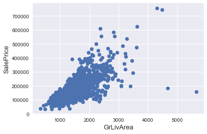
Documentation for the Ames Housing Data indicates that there are outliers present in the training data 1: http://ww2.amstat.org/publications/jse/v19n3/Decock/DataDocumentation.txt

Let’s explore these outliers

fig, ax = plt.subplots()
ax.scatter(x = train['GrLivArea'], y = train['SalePrice'])
plt.ylabel('SalePrice', fontsize=13)
plt.xlabel('GrLivArea', fontsize=13)
plt.show()

We can see at the bottom right two with extremely large GrLivArea that are of a low price. These values are huge oultliers. Therefore, we can safely delete them.

Note :

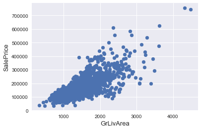
Outliers removal is not always safe. We decided to delete these two as they are very huge and really bad ( extremely large areas for very low prices).

There are probably others outliers in the training data. However, removing all them may affect badly our models if ever there were also outliers in the test data. That’s why , instead of removing them all, we will just manage to make some of our models robust on them. You can refer to the modelling part of this notebook for that.

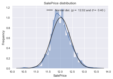
Target Variable

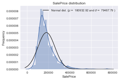
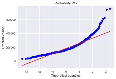
SalePrice is the variable we need to predict. So let’s do some analysis on this variable first.

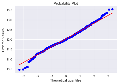
The target variable is right skewed. As (linear) models love normally distributed data , we need to transform this variable and make it more normally distributed.

Log-transformation of the target variable

The skew seems now corrected and the data appears more normally distributed.

Features engineering

let’s first concatenate the train and test data in the same dataframe

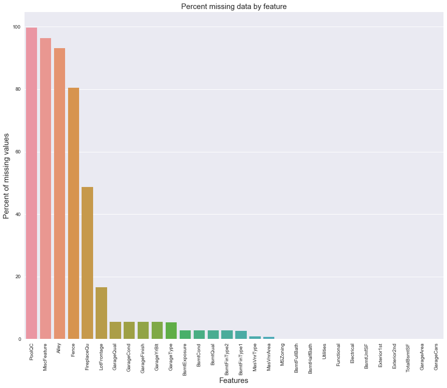
Missing Data

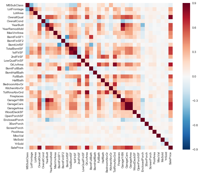
Data Correlation

Imputing missing values

We impute them by proceeding sequentially through features with missing values

• PoolQC : data description says NA means “No Pool”. That make sense, given the huge ratio of missing value (+99%) and majority of houses have no Pool at all in general.

all_data["PoolQC"] = all_data["PoolQC"].fillna("None")

• MiscFeature : data description says NA means “no misc feature”

all_data["MiscFeature"] = all_data["MiscFeature"].fillna("None")

• Alley : data description says NA means “no alley access”

all_data["Alley"] = all_data["Alley"].fillna("None")

• Fence : data description says NA means “no fence”

all_data["Fence"] = all_data["Fence"].fillna("None")

• FireplaceQu : data description says NA means “no fireplace”

all_data["FireplaceQu"] = all_data["FireplaceQu"].fillna("None")

• LotFrontage : Since the area of each street connected to the house property most likely have a similar area to other houses in its neighborhood , we can fill in missing values by the median LotFrontage of the neighborhood.

#Group by neighborhood and fill in missing value by the median LotFrontage of all the neighborhood
all_data["LotFrontage"] = all_data.groupby("Neighborhood")["LotFrontage"].transform(
    lambda x: x.fillna(x.median()))

• GarageType, GarageFinish, GarageQual and GarageCond : Replacing missing data with None

for col in ('GarageType', 'GarageFinish', 'GarageQual', 'GarageCond'):
    all_data[col] = all_data[col].fillna('None')

• GarageYrBlt, GarageArea and GarageCars : Replacing missing data with 0 (Since No garage = no cars in such garage.)

for col in ('GarageYrBlt', 'GarageArea', 'GarageCars'):
    all_data[col] = all_data[col].fillna(0)

• BsmtFinSF1, BsmtFinSF2, BsmtUnfSF, TotalBsmtSF, BsmtFullBath and BsmtHalfBath : missing values are likely zero for having no basement

for col in ('BsmtFinSF1', 'BsmtFinSF2', 'BsmtUnfSF','TotalBsmtSF', 'BsmtFullBath', 'BsmtHalfBath'):
    all_data[col] = all_data[col].fillna(0)

• BsmtQual, BsmtCond, BsmtExposure, BsmtFinType1 and BsmtFinType2 : For all these categorical basement-related features, NaN means that there is no basement.

for col in ('BsmtQual', 'BsmtCond', 'BsmtExposure', 'BsmtFinType1', 'BsmtFinType2'):
    all_data[col] = all_data[col].fillna('None')

• MasVnrArea and MasVnrType : NA most likely means no masonry veneer for these houses. We can fill 0 for the area and None for the type.

all_data["MasVnrType"] = all_data["MasVnrType"].fillna("None")
all_data["MasVnrArea"] = all_data["MasVnrArea"].fillna(0)

• MSZoning (The general zoning classification) : ‘RL’ is by far the most common value. So we can fill in missing values with ‘RL’

all_data['MSZoning'] = all_data['MSZoning'].fillna(all_data['MSZoning'].mode()[0])

• Utilities : For this categorical feature all records are “AllPub”, except for one “NoSeWa” and 2 NA . Since the house with ‘NoSewa’ is in the training set, this feature won’t help in predictive modelling. We can then safely remove it.

all_data = all_data.drop(['Utilities'], axis=1)

• Functional : data description says NA means typical

all_data["Functional"] = all_data["Functional"].fillna("Typ")

• Electrical : It has one NA value. Since this feature has mostly ‘SBrkr’, we can set that for the missing value.

all_data['Electrical'] = all_data['Electrical'].fillna(all_data['Electrical'].mode()[0])

• KitchenQual: Only one NA value, and same as Electrical, we set ‘TA’ (which is the most frequent) for the missing value in KitchenQual.

all_data['KitchenQual'] = all_data['KitchenQual'].fillna(all_data['KitchenQual'].mode()[0])

• Exterior1st and Exterior2nd : Again Both Exterior 1 & 2 have only one missing value. We will just substitute in the most common string

all_data['Exterior1st'] = all_data['Exterior1st'].fillna(all_data['Exterior1st'].mode()[0])
all_data['Exterior2nd'] = all_data['Exterior2nd'].fillna(all_data['Exterior2nd'].mode()[0])

• SaleType : Fill in again with most frequent which is “WD”

all_data['SaleType'] = all_data['SaleType'].fillna(all_data['SaleType'].mode()[0])

• MSSubClass : Na most likely means No building class. We can replace missing values with None

all_data['MSSubClass'] = all_data['MSSubClass'].fillna("None")

Is there any remaining missing value ?

It remains no missing value.

More features engeneering

Transforming some numerical variables that are really categorical

Label Encoding some categorical variables that may contain information in their ordering set

Adding one more important feature

Since area related features are very important to determine house prices, we add one more feature which is the total area of basement, first and second floor areas of each house

Skewed features

Box Cox Transformation of (highly) skewed features

We use the scipy function boxcox1p which computes the Box-Cox transformation of \(1 + x\).

Note that setting \( \lambda = 0 \) is equivalent to log1p used above for the target variable.

See this page for more details on Box Cox Transformation as well as [the scipy function’s page]2: http://onlinestatbook.com/2/transformations/box-cox.html [2]: https://docs.scipy.org/doc/scipy-0.19.0/reference/generated/scipy.special.boxcox1p.html

There are 59 skewed numerical features to Box Cox transform

Modelling

In this approach, we add a meta-model on averaged base models and use the out-of-folds predictions of these base models to train our meta-model.

The procedure, for the training part, may be described as follows:

1. Split the total training set into two disjoint sets (here train and .holdout )

2. Train several base models on the first part (train)

3. Test these base models on the second part (holdout)

4. Use the predictions from 3) (called out-of-folds predictions) as the inputs, and the correct responses (target variable) as the outputs to train a higher level learner called meta-model.

The first three steps are done iteratively . If we take for example a 5-fold stacking , we first split the training data into 5 folds. Then we will do 5 iterations. In each iteration, we train every base model on 4 folds and predict on the remaining fold (holdout fold).

So, we will be sure, after 5 iterations , that the entire data is used to get out-of-folds predictions that we will then use as new feature to train our meta-model in the step 4.

For the prediction part , We average the predictions of all base models on the test data and used them as meta-features on which, the final prediction is done with the meta-model.

(Image taken from Faron)

Gif taken from KazAnova’s interview

On this gif, the base models are algorithms 0, 1, 2 and the meta-model is algorithm 3. The entire training dataset is A+B (target variable y known) that we can split into train part (A) and holdout part (B). And the test dataset is C.

B1 (which is the prediction from the holdout part) is the new feature used to train the meta-model 3 and C1 (which is the prediction from the test dataset) is the meta-feature on which the final prediction is done.

Define a cross validation strategy

We use the cross_val_score function of Sklearn. However this function has not a shuffle attribut, we add then one line of code, in order to shuffle the dataset prior to cross-validation

Base models

• LASSO Regression :

This model may be very sensitive to outliers. So we need to made it more robust on them. For that we use the sklearn’s Robustscaler() method on pipeline

lasso = make_pipeline(RobustScaler(), Lasso(alpha =0.0005, random_state=1))

• Elastic Net Regression :

again made robust to outliers

ENet = make_pipeline(RobustScaler(), ElasticNet(alpha=0.0005, l1_ratio=.9, random_state=3))

• Kernel Ridge Regression :

KRR = KernelRidge(alpha=0.6, kernel='polynomial', degree=2, coef0=2.5)

• Gradient Boosting Regression :

With huber loss that makes it robust to outliers

GBoost = GradientBoostingRegressor(n_estimators=3000, learning_rate=0.05,
                                   max_depth=4, max_features='sqrt',
                                   min_samples_leaf=15, min_samples_split=10, 
                                   loss='huber', random_state =5)

• XGBoost :

#EDIT: changing the xgboost parameters for better CV score

#model_xgb = xgb.XGBRegressor(colsample_bytree=0.2, gamma=0.0, 
#                            learning_rate=0.05, max_depth=6, 
#                             min_child_weight=1.5, n_estimators=7200,
#                             reg_alpha=0.9, reg_lambda=0.6,
#                             subsample=0.2,seed=42, silent=1,
#                             random_state =7)

model_xgb = xgb.XGBRegressor(colsample_bytree=0.4603, gamma=0.0468, 
                             learning_rate=0.05, max_depth=3, 
                             min_child_weight=1.7817, n_estimators=2200,
                             reg_alpha=0.4640, reg_lambda=0.8571,
                             subsample=0.5213, silent=1,
                              nthread = -1)

• LightGBM :

model_lgb = lgb.LGBMRegressor(objective='regression',num_leaves=5,
                              learning_rate=0.05, n_estimators=720,
                              max_bin = 55, bagging_fraction = 0.8,
                              bagging_freq = 5, feature_fraction = 0.2319,
                              feature_fraction_seed=9, bagging_seed=9,
                              min_data_in_leaf =6, min_sum_hessian_in_leaf = 11)

Base models scores

Let’s see how these base models perform on the data by evaluating the cross-validation rmsle error

score = rmsle_cv(lasso)
print("\nLasso score: {:.4f} ({:.4f})\n".format(score.mean(), score.std()))

1

Lasso score: 0.1115 (0.0074)

score = rmsle_cv(ENet)
print("ElasticNet score: {:.4f} ({:.4f})\n".format(score.mean(), score.std()))

1

ElasticNet score: 0.1116 (0.0074)

score = rmsle_cv(KRR)
print("Kernel Ridge score: {:.4f} ({:.4f})\n".format(score.mean(), score.std()))

1

Kernel Ridge score: 0.1153 (0.0075)

score = rmsle_cv(GBoost)
print("Gradient Boosting score: {:.4f} ({:.4f})\n".format(score.mean(), score.std()))

1

Gradient Boosting score: 0.1177 (0.0080)

score = rmsle_cv(model_xgb)
print("Xgboost score: {:.4f} ({:.4f})\n".format(score.mean(), score.std()))

1

Xgboost score: 0.1149 (0.0059)

score = rmsle_cv(model_lgb)
print("LGBM score: {:.4f} ({:.4f})\n" .format(score.mean(), score.std()))

1

LGBM score: 0.1151 (0.0055)

class AveragingModels(BaseEstimator, RegressorMixin, TransformerMixin):
    def __init__(self, models):
        self.models = models
        
    # we define clones of the original models to fit the data in
    def fit(self, X, y):
        self.models_ = [clone(x) for x in self.models]
        
        # Train cloned base models
        for model in self.models_:
            model.fit(X, y)

        return self
    
    #Now we do the predictions for cloned models and average them
    def predict(self, X):
        predictions = np.column_stack([
            model.predict(X) for model in self.models_
        ])
        return np.mean(predictions, axis=1)   

averaged_models = AveragingModels(models = (ENet, GBoost, KRR, lasso))

score = rmsle_cv(averaged_models)
print(" Averaged base models score: {:.4f} ({:.4f})\n".format(score.mean(), score.std()))

1

 Averaged base models score: 0.1091 (0.0075)

class StackingAveragedModels(BaseEstimator, RegressorMixin, TransformerMixin):
    def __init__(self, base_models, meta_model, n_folds=5):
        self.base_models = base_models
        self.meta_model = meta_model
        self.n_folds = n_folds
   
    # We again fit the data on clones of the original models
    def fit(self, X, y):
        self.base_models_ = [list() for x in self.base_models]
        self.meta_model_ = clone(self.meta_model)
        kfold = KFold(n_splits=self.n_folds, shuffle=True, random_state=156)
        
        # Train cloned base models then create out-of-fold predictions
        # that are needed to train the cloned meta-model
        out_of_fold_predictions = np.zeros((X.shape[0], len(self.base_models)))
        for i, model in enumerate(self.base_models):
            for train_index, holdout_index in kfold.split(X, y):
                instance = clone(model)
                self.base_models_[i].append(instance)
                instance.fit(X[train_index], y[train_index])
                y_pred = instance.predict(X[holdout_index])
                out_of_fold_predictions[holdout_index, i] = y_pred
                
        # Now train the cloned  meta-model using the out-of-fold predictions as new feature
        self.meta_model_.fit(out_of_fold_predictions, y)
        return self
   
    #Do the predictions of all base models on the test data and use the averaged predictions as 
    #meta-features for the final prediction which is done by the meta-model
    def predict(self, X):
        meta_features = np.column_stack([
            np.column_stack([model.predict(X) for model in base_models]).mean(axis=1)
            for base_models in self.base_models_ ])
        return self.meta_model_.predict(meta_features)

stacked_averaged_models = StackingAveragedModels(base_models = (ENet, GBoost, KRR),
                                                 meta_model = lasso)

score = rmsle_cv(stacked_averaged_models)
print("Stacking Averaged models score: {:.4f} ({:.4f})".format(score.mean(), score.std()))

1

Stacking Averaged models score: 0.1085 (0.0074)

def rmsle(y, y_pred):
    return np.sqrt(mean_squared_error(y, y_pred))

stacked_averaged_models.fit(train.values, y_train)
stacked_train_pred = stacked_averaged_models.predict(train.values)
stacked_pred = np.expm1(stacked_averaged_models.predict(test.values))
print(rmsle(y_train, stacked_train_pred))

1

0.0781571937916

model_xgb.fit(train, y_train)
xgb_train_pred = model_xgb.predict(train)
xgb_pred = np.expm1(model_xgb.predict(test))
print(rmsle(y_train, xgb_train_pred))

1

0.0785366603111

model_lgb.fit(train, y_train)
lgb_train_pred = model_lgb.predict(train)
lgb_pred = np.expm1(model_lgb.predict(test.values))
print(rmsle(y_train, lgb_train_pred))

1

0.0722556085687

'''RMSE on the entire Train data when averaging'''

print('RMSLE score on train data:')
print(rmsle(y_train,stacked_train_pred*0.70 +
               xgb_train_pred*0.15 + lgb_train_pred*0.15 ))

1
2

RMSLE score on train data:
0.0753189601002

ensemble = stacked_pred*0.70 + xgb_pred*0.15 + lgb_pred*0.15

sub = pd.DataFrame()
sub['Id'] = test_ID
sub['SalePrice'] = ensemble
sub.to_csv('submission.csv',index=False)